Google Sheets Alternate Row Color for sheet cell

Benefits of Alternating Color in Google Sheets

After completing the calculation and data entry work, the next step we will do is to format the colors and fonts to make the data table more beautiful and clear. That is the reason why we should color alternately to make it easier to read the data. Google Sheets supports many different ways to format alternating colors for data tables such as choosing alternate colors or conditional color formatting.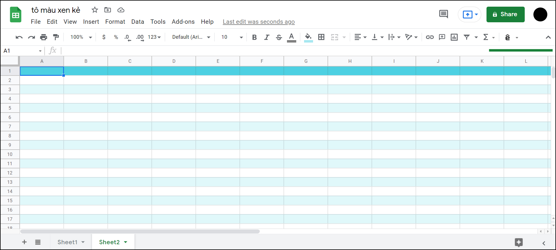

How to color alternately in Google Sheets using "Alternating Colors"

Step 1: Select the data area to color > Select Format > Select Alternating colors.

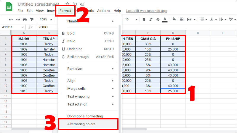
Go to Formart and Select Alternating colors

Step 2: Select a default style > Click Done.

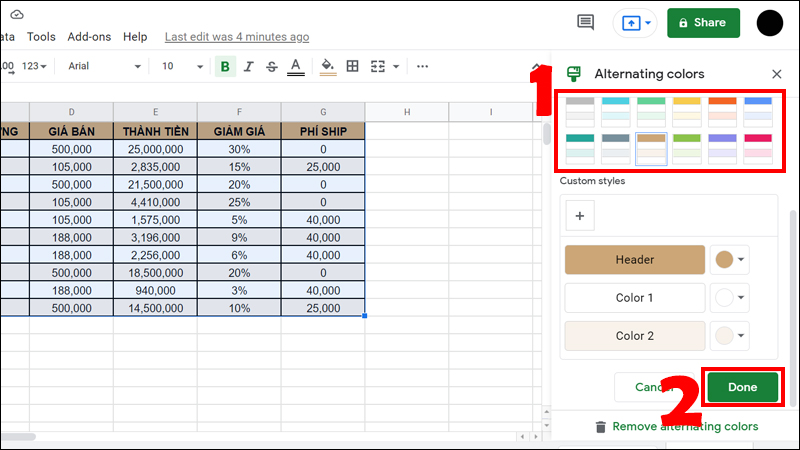
Select a default style

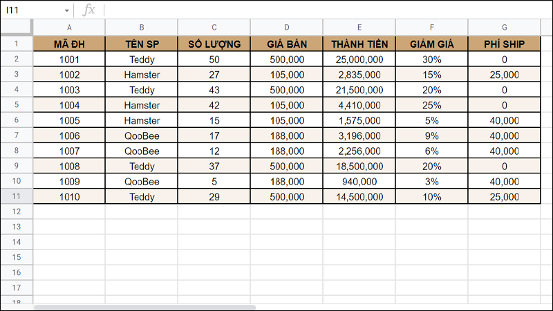
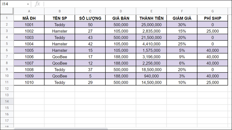
Result after selecting an alternative color.

How to color alternately in Google Sheets using a function

Before performing the function to color alternately, you will perform the following steps: Select the data area to color > Select Format > Select Conditional formatting.

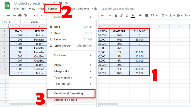
Select Format and select Conditional formatting

How to color alternate rows in Google Sheets

Select Custom formula is > Enter the formula: =ISEVEN(ROW()) > Select the color you want to color > Click Done.

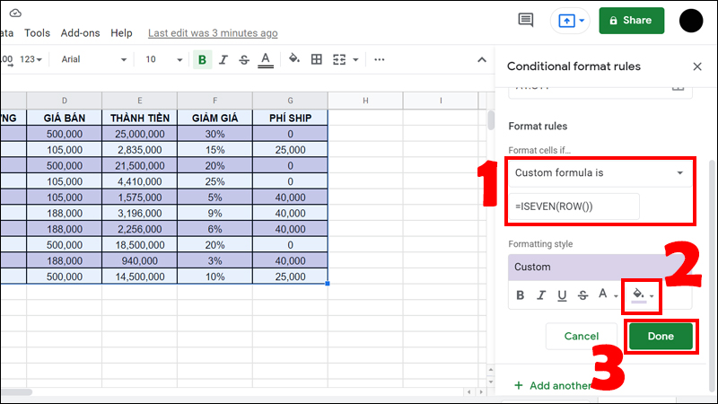
Enter the formula, select the color you want to fill and press Done

The resulting color is filled in alternating rows.

How to color arbitrary rows in Google Sheets

Enter the formula: =MOD(ROW();5)=0 > Select the color you want to color > Click Done.

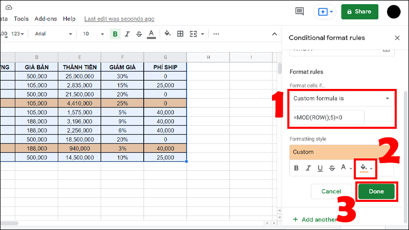
Enter the formula, select the color you want to fill and press Done

The result will be 5 lines of color 1 time. You can change the number of lines to fill the color.

How to color alternating columns in Google Sheets

Enter the formula: =ISEVEN(COLUMN()) > Select the color you want to color > Click Done.

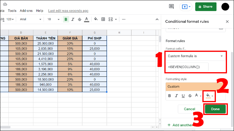
Enter the formula, select the color you want to fill and press Done

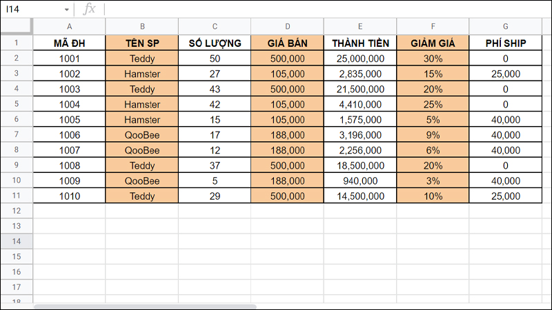
The resulting color is filled in alternating columns.

How to color custom columns in Google Sheets

Enter the formula: =MOD(COLUMN();3)=0 > Select the color you want to color > Click Done.

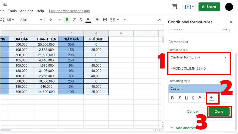
Enter the formula, select the color you want to fill and press Done

The result will be filled every 3 columns of color. You can change the number of columns to fill.

Some related questions

How to filter by color in Google Sheets?

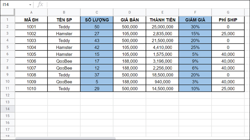
Step 1: Select the data area you want to filter > Select the Filter icon.

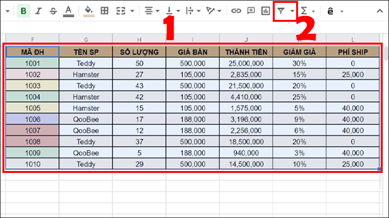
Select the data area you want to filter and Select the Filter icon

Step 2: Select the arrow in the first row of the data area with the color you want to filter > Select Filter by color > Select Fill Color > Select the color you want to filter.

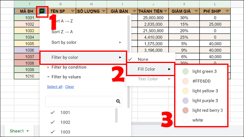
Select Fill Color and Select the color you want to filter

How to remove the applied coloring rule?

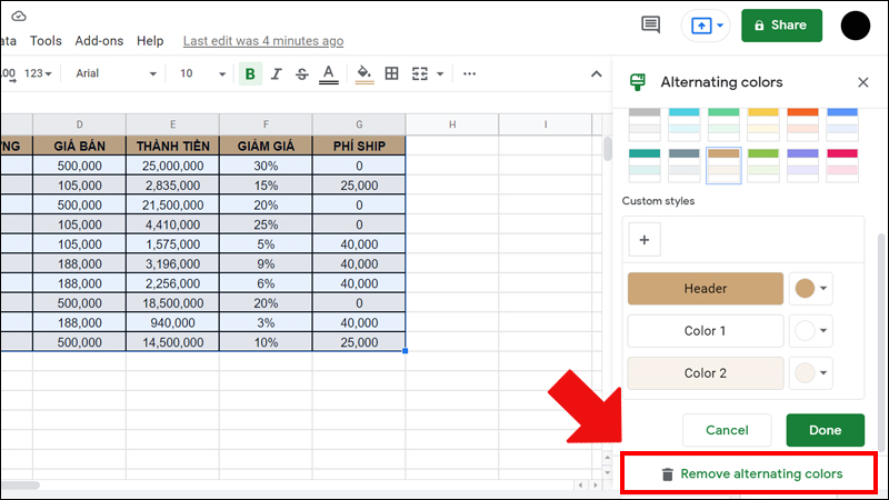
• Case 1: Remove the alternate color.

The steps to remove the alternate color are similar to the instructions in section 2. Select the data area to be colored > Select Format > Select Alternating colors > Select Remove alternating colors.

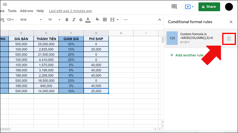
• Case 2: Delete the custom formula.

The steps to delete the replacement color are similar to the instructions in section 3. Select the data area to be colored > Select Format > Select Conditional formatting > Click the trash can icon to delete the formula.

How to color alternately in Google Sheets on mobile?

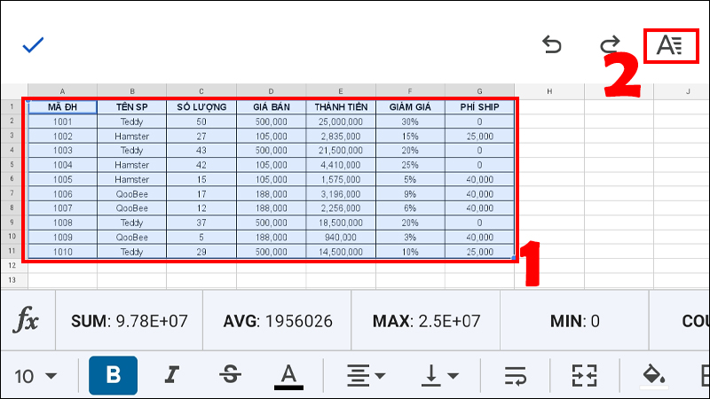
Step 1: Highlight the data area > Click on the format icon (letter A) in the upper right corner.

Step 2: Select the Cells tab > Select Conditional Formatting or Alternate Colors. Then follow the same steps as on the computer.

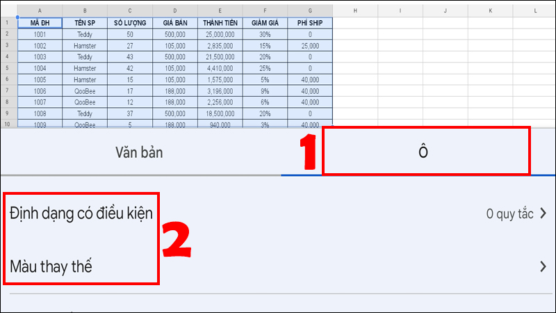
Select the Cells tab and select Conditional Formatting or Alternate Colors